July 25, 2012

I looked into Fourier transforms of bias data, based on reports (see ​http://asd.gsfc.nasa.gov/Bernard.Rauscher/Research/Publications_files/article.pdf) that the read noise can be improved via a Fourier process. The method described assumes that the correlated noise arises due to a time dependent component that is difficult to detect. Therefore, in order to examine this, I asked Sidik for the read out times that could be used to flag each pixel with a given time. Sidik responded that the pixels are read out as

 T(x,y) = x * dt + y * (dt2 + e2 + delta2)

where x and y are the pixel coordinates on a cell, dt is the readout time for a pixel (dt = 2030ns), dt2 is the time to shift rows down (dt2 = 89880ns), e2 is a constant unknown error in dt2 (e2 <= 100ns), and delta2 is a jitter component (delta2 = +/- 10-20ns). As e2 and delta2 are small relative to dt2, they were ignored entirely.

To prepare the pixel data to allow for an FFT, the image mean was subtracted (to zero the DC component), and the pixels were indexed based on dt, such that

 i(x,y) = x + int(y * 89880 / 2030) / y

with all unpopulated values of i zero-padded.

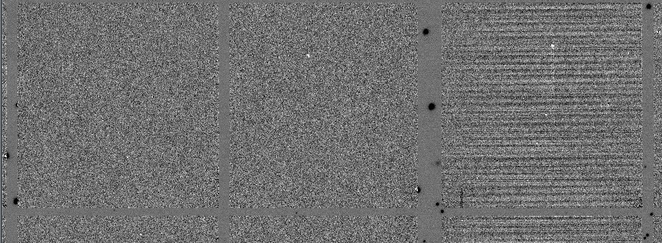
Two OTAs were chosen for study, OTA33 (the "good" OTA), and OTA67 (the "bad" OTA). These two were selected based on the row-by-row bias properties that have been noticed before. A variety of cells on the OTA were checked, all of which seem to have similar results, so cell xy01 is presented here. A bias exposure was selected more or less at random, and the FFT calculated.

Results?

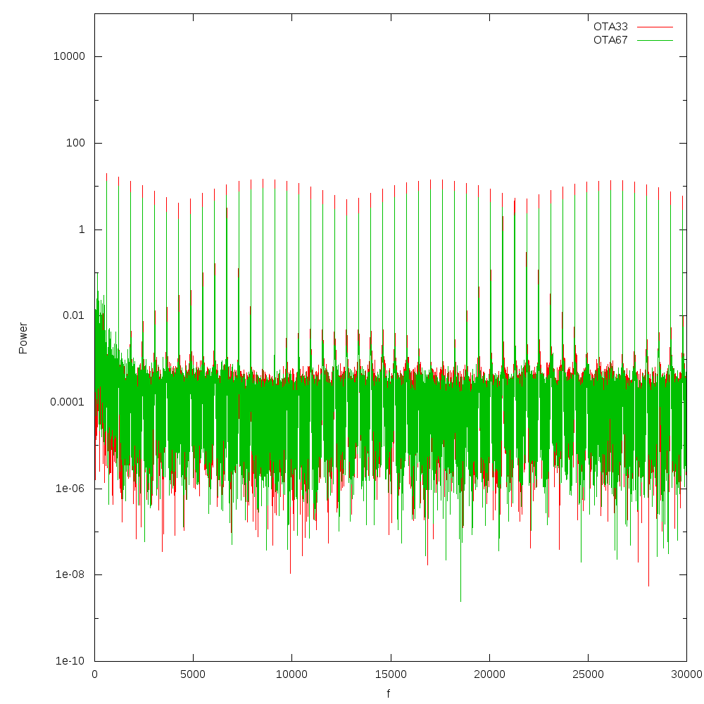
This image shows a selection of the FFT power for a section of the lowest frequencies. The spikes correspond with the ~600 pixel spacing of rows.

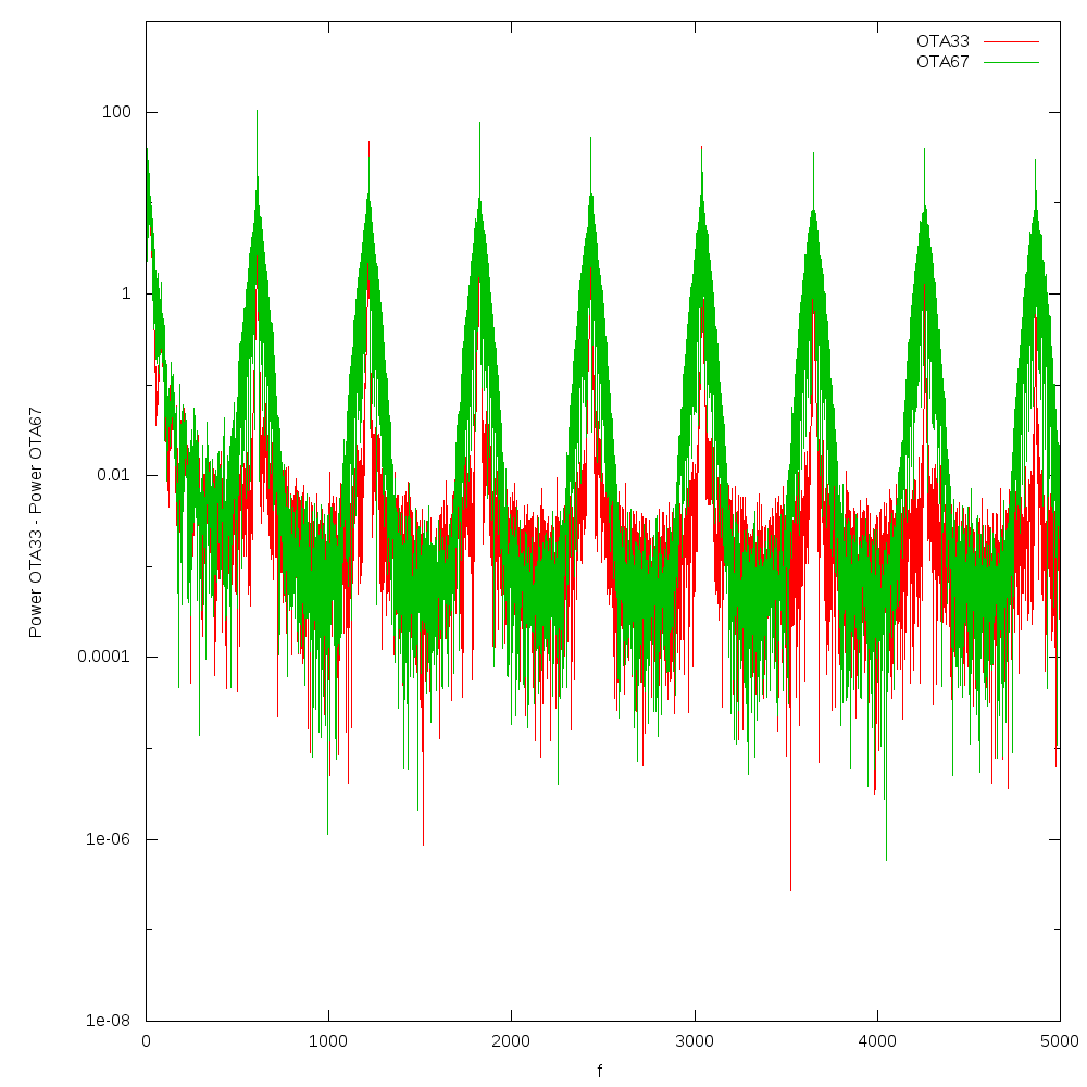
Zooming in on the lowest frequencies shows that there is basically no difference between the bias from OTA33 and the bias from OTA67. No clear "row-to-row" noise signal seems to pop up, although it is somewhat clear that the 600-pixel spike peaks are lower in the OTA67 bias, suggesting that some of that power is dispersed among other frequencies.

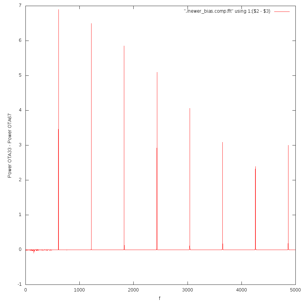
The difference in the power, showing that other than the difference in spike peaks, the two signals are very similar.

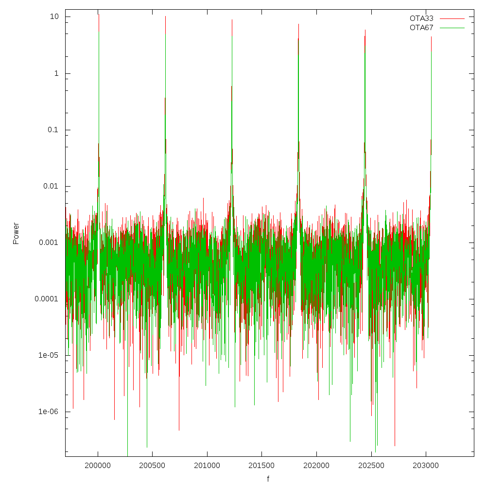
Repeating the experiment with a science image instead of a bias. The y-axis is again Power, not the difference. For the science images, at low frequencies, the spikes are spread out on OTA67 compared to OTA33.

This effect is minimal at the highest frequencies, suggesting that in science images, there is a difference in the low frequency.

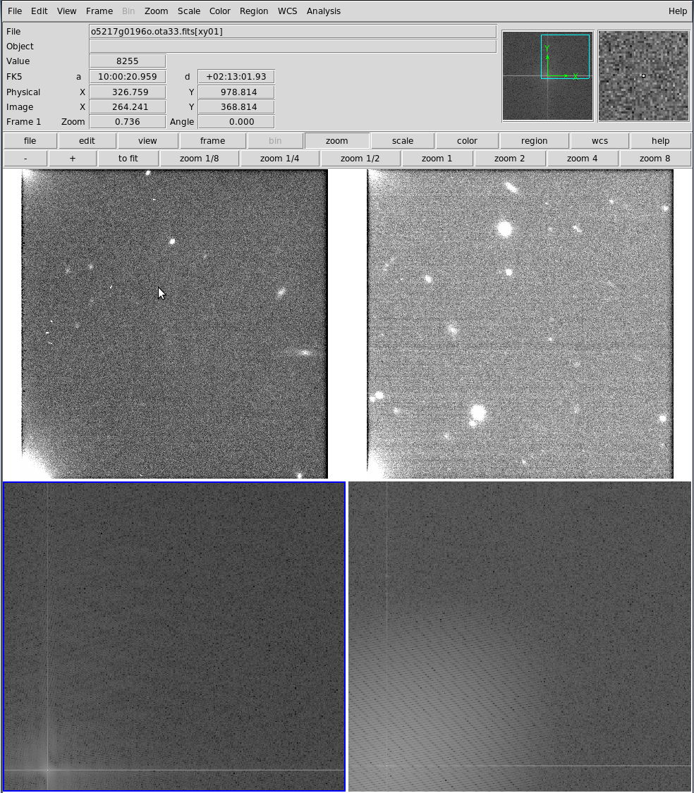
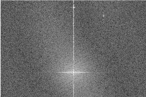
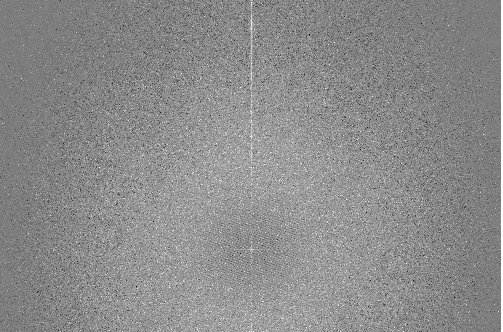
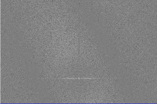
To satisfy my own curiosity, I calculated the 2d image power. Clockwise from top left, this shows the OTA33 bias, the OTA67 bias, the power in one quadrant of the OTA67 FFT, and the same quadrant of the OTA33 FFT (zero frequencies are at the cross center in the lower left). These images show a similar result to the 1d-FFTs. The spikes that we see in the 1d FFT corresponds with the vertical bar at f_x = 0. Although this bar does spread out in some places (corresponding to the row-to-row structure visible in the bias), there is again no major difference.

Same arrangement of images for a science image. This is somewhat complicated by the fact that astronomical sources do have some effect on the output FFT. However, it is clear that the low-frequency region for OTA67 has significantly more power than the same region in OTA33.